機器學習可以從數據中得到有用的見解. 目標是縱觀Spark MLlib,采取適合的算法從數據集中生偏見解。對 Twitter的數據集, 采取非監督集群算法來辨別與Apache?Spark相干的tweets . 初始輸入是混合在1起的tweets。 首先提取相干特性, 然后在數據集中使用機器學習算法 , 最后評估結果和性能.
?本章重點以下:
???了解 Spark MLlib 模塊及其算法,還有典型的機器學習流程 .
???? 預處理 所收集的Twitter 數據集提取相干特性, 利用非監督集群算法辨認Apache Spark-?相干的tweets. 然后, 評估得到的模型和結果.
????? 描寫Spark 機器學習的流水線
Spark MLlib 在利用架構中的位置
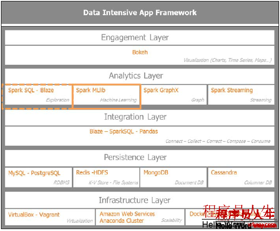
先看1下數據學習在數據密集型利用架構中的位置,集中關注分析層,準確1點說是機器學習。這是批處理和流處理數據學習的基礎,它們只是推測的規則不同。
?下圖指出了重點, 分析層處理的探索式數據分析工具 Spark SQL和Pandas外 還有機器學習模塊.?
?
Spark MLlib 算法分類
Spark MLlib 是1個更新很快的模塊,新的算法不斷地引入到 Spark中.
下圖提供了 Spark MLlib 算法的高層通覽,并根據傳統機器學習技術的體系或數據的連續性進行了分組:
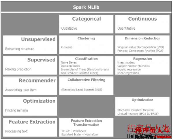
根據數據的類型,將 Spark MLlib 算法分成兩欄, 性質無序或數量連續的 . 我們將數據辨別為無序的性質數據和數量連續的數據。1個性質數據的例子:在給定大氣壓,溫度,云的類型和顯現, 天氣是晴朗,干燥,多雨,或陰天時?時,預測她是不是穿著男性上裝,這是離散的值。 另外一方面, 給定了位置,住房面積,房間數,想預測房屋的價格 , 房地產可以通過線性回歸預測。 ?本例中,討論數量連續的數據。
水平分組反應了所使用的機器學習算法的類型。監督和非監督機器學習取決于訓練的數據是不是標注。非監督學習的挑戰是對非標注數據使用學習算法。目標是發現輸入中隱含的結構。?而監督式學習的數據是標注過的。 重點是對連續數據的回歸預測和離散數據的分類.
?機器學習的1個重要門類是推薦系統,主要是利用了協同過濾技術。 Amazon 和 Netflix 有自己非常強大的 推薦系統.?? 隨機梯度降落是合適于Spark散布計算的機器學習優化技術之1。對處理大量的文本,Spark提供了特性提取和轉換的重要的庫例如: TF-IDF , Word2Vec, standard scaler, 和normalizer.??
監督和非監督式學習
深入研究1下Spark MLlib 提供的傳統的機器學習算法 . 監督和非監督機器學習取決于訓練的數據是不是標注. 區分無序和連續取決于數據的離散或連續.
下圖解釋了 Spark MLlib 監督和非監督時算法及預處理技術 :
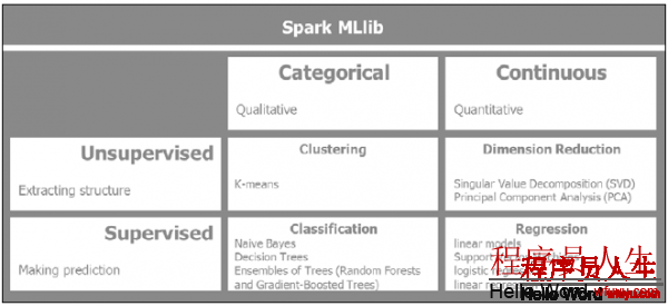
下面時Spakr MLlib中的監督和非監督算法和與預處理技術:
?? Clustering 聚類: 1個非監督式機器學習技術,數據是沒有標注的,目的是數據中提取結構:?
?∞ K-Means: 從 K個不同聚類中進行數據分片
??∞ Gaussian Mixture: 基于組件的最大化后驗幾率聚類
???∞ Power Iteration Clustering(PIC): 根據圖頂點的兩兩邊的類似程度聚類?
???∞ Latent Dirichlet Allocation (LDA): 用于將文本文檔聚類成話題
????∞ Streaming K-Means: 使用窗口函數將進入的數據活動態的進行K-Means聚類?
? Dimensionality Reduction: 目的在減少特性的數量. 基本上, 用于削減數據噪音并關注關鍵特性:?
∞ Singular Value Decomposition (SVD): 將矩陣中的數據分割成簡單的成心義的小片,把初始矩陣生成3個矩陣.
∞ Principal Component Analysis (PCA): 以子空間的低維數據逼近高維數據集..
? Regression and Classification: 當分類器將結果分成類時,回歸使用標注過的訓練數據來預測輸出結果。分類的變量是離散無序的,回歸的變量是連續而有序的?:?
∞
Linear Regression Models (linear regression, logistic regression,?
and support vector machines): 線性回歸算法可以表達為凸優化問題,目的是基于有權重變量的向量使目標函數最小化. 目標函數通過函數的
正則部份控制函數的復雜性,通過函數的損失部份控制函數的誤差.?
∞
Naive Bayes: 基于給定標簽的條件幾率來預測,基本假定是變量的相互獨立性。
?∞
Decision Trees: 它履行了特性空間的遞歸2元劃分,為了最好的劃分分割需要將樹狀節點的信息增益最大化。
??∞
Ensembles of trees (
Random Forests and Gradient-
Boosted Trees):?樹集成算法結合了多種決策樹模型來構建1個高性能的模型,它們對分類和回歸是非常直觀和成功的。?
? Isotonic Regression保序回歸: 最小化所給數據和可觀測響應的均方根誤差.
其他學習算法
?Spark MLlib 還提供了很多其它的算法,廣泛地說有3種其它的機器學習算法:
推薦系統, 優化算法, 和特點提取.
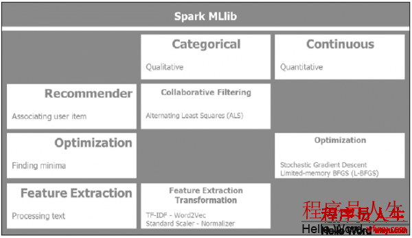
下面當前是 MLlib 中的其它算法:
?? Collaborative filtering: 是推薦系統的基礎,創建用戶-物品關聯矩陣,目標是填充差異。基于其它用戶與物品的關聯評分,為沒有評分的目標用戶推薦物品。在散布式計算中, ALS (Alternating Least Square)是最成功的算法之1:?
?∞ Alternating Least Squares交替最小2乘法: 矩陣分解技術采取了隱性反饋,時間效應和置信水平,把大范圍的用戶物品矩陣分解成低維的用戶物品因子,通過替換因子最小化2次損失函數。
??? Feature extraction and transformation: 這些是大范圍文檔處理的基礎,包括以下技術:
∞ Term Frequency: 搜素引擎使用Search engines use TF-IDF 對語料庫中的文檔進行等級評分。機器學習中用它來判斷1個詞在文檔或語料庫中的重要性. 詞頻統計所肯定的權重取決于它在語料庫中出現的頻率。 詞頻本身可能存在毛病導向比如過分強調了類似 the, of, or and 等這樣無意義的信息辭匯. 逆文檔頻率提供了特異性或信息量的度量,辭匯在語料庫中所有文檔是不是常見。
∞ Word2Vec: 包括了兩個模型 Skip-Gram 和Continuous? Bag of Word. Skip-Gram 預測了1個給定辭匯的鄰近詞, 基于辭匯的滑動窗口; Continuous Bag of?Words 預測了所給定鄰近辭匯確當前詞是甚么.
?∞ Standard Scaler: 作為預處理的1部份,數據集常常通過平均去除和方差縮放來標準化. 我們在訓練數據上計算平均和標準偏差,并利用一樣的變形來測試數據.
??∞ Normalizer: 在縮放樣本時需要規范化. 對點積或核心方法這樣的2次型非常有用。
?∞ Feature selection: 通過選擇模型中最相干的特點來下降向量空間的維度。
??∞ Chi-Square Selector: 1個統計方法來丈量兩個事件的獨立性。
? Optimization: 這些 Spark MLlib 優化算法聚焦在各種梯度降落的技術。 Spark 在散布式集群上提供了非常有效的梯度降落的實現,通過本地極小的迭代完成梯度的快速降落。迭代所有的數據變量是計算密集型的:?
∞ Stochastic Gradient Descent: 最小化目標函數即?微分函數的和. 隨機梯度降落僅使用了1個訓練數據的抽樣來更新1個特殊迭代的參數,用來解決大范圍稀疏機器學習問題例如文本分類.?
? Limited-memory BFGS (L-BFGS): 文如其名,L-BFGS使用了有限內存,合適于Spark MLlib 實現的散布式優化算法。?
Spark MLlib data types
?MLlib 支持4種數據類型: local vector, labeled point, local matrix,?and distributed matrix. Spark MLlib 算法廣泛地使用了這些數據類型:
??? Local vector: 位于單機,可以是緊密或稀疏的:?
??∞ Dense vector 是傳統的 doubles 數組. 例如[5.0, 0.0, 1.0, 7.0].?
??∞ Sparse vector 使用整數和double值. 稀疏向量 [5.0, 0.0, 1.0, 7.0] 應當是 (4,?[0, 2, 3], [5.0, 1.0, 7.0]),表明了向量的維數.
這是 PySpark中1個使用本地向量的例子:
import numpy as np
import scipy.sparse as sps
from pyspark.mllib.linalg import Vectors # NumPy array for dense vector. dvect1 = np.array([5.0, 0.0, 1.0, 7.0]) # Python list for dense vector. dvect2 = [5.0, 0.0, 1.0, 7.0] # SparseVector creation svect1 = Vectors.sparse(4, [0, 2, 3], [5.0, 1.0, 7.0]) # Sparse vector using a single-column SciPy csc_matrix svect2 = sps.csc_matrix((np.array([5.0, 1.0, 7.0]), np.array([0, 2, 3])), shape = (4, 1))
? Labeled point. 1個標注點是監督式學習中的1個有標簽的緊密或稀疏向量. 在2元標簽中, 0.0 代表負值, 1.0 代表正值.?
這有1個PySpark中標注點的例子:
from pyspark.mllib.linalg import SparseVector
from pyspark.mllib.regression import LabeledPoint
# Labeled point with a positive label and a dense feature vector.
lp_pos = LabeledPoint(1.0, [5.0, 0.0, 1.0, 7.0])
# Labeled point with a negative label and a sparse feature vector.
lp_neg = LabeledPoint(0.0, SparseVector(4, [0, 2, 3], [5.0, 1.0, 7.0]))
? Local Matrix: 本地矩陣位于單機上,具有整型索引和double的值.
這是1個 PySpark中本地矩陣的例子:
from pyspark.mllib.linalg import Matrix, Matrices # Dense matrix ((1.0, 2.0, 3.0), (4.0, 5.0, 6.0)) dMatrix = Matrices.dense(2, 3, [1, 2, 3, 4, 5, 6]) # Sparse matrix ((9.0, 0.0), (0.0, 8.0), (0.0, 6.0)) sMatrix = Matrices.sparse(3, 2, [0, 1, 3], [0, 2, 1], [9, 6, 8])
? Distributed Matrix: 充分利用 RDD的成熟性,散布式矩陣可以在集群中同享?. 有4種散布式矩陣類型: RowMatrix, IndexedRowMatrix,?CoordinateMatrix, 和 BlockMatrix:
?∞ RowMatrix: 使用多個向量的1個 RDD,創建無意義索引的行散布式矩陣叫做 RowMatrix.
??∞ IndexedRowMatrix: 行索引是成心義的. 首先使用IndexedRow 類創建1個 帶索引行的RDDFirst,?再創建1個 IndexedRowMatrix.
???∞ CoordinateMatrix: 對表達巨大而稀疏的矩陣非常有用。CoordinateMatrix 從MatrixEntry的RDD創建,用類型元組 (long, long, or float)來表示。
????∞ BlockMatrix: 從 子矩陣塊的RDDs創建,?子矩陣塊形如 ((blockRowIndex, blockColIndex),?sub-matrix).?
機器學習的工作流和數據流
?
?除算法, 機器學習還需要處理進程,我們將討論監督和非監督學習的典型流程和數據流.??
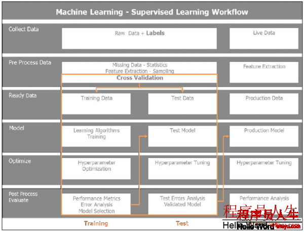
監督式學習工作流程
在監督式學習中, 輸入的訓練數據集是標注過的. 1個重要的話數據實踐是分割輸入來訓練和測試, 和嚴重相應的模式.完成監督式學習有6個步驟:
? Collect the data: 這個步驟依賴于前面的章節,保證數據正確的容量和顆粒度,使機器學習算法能夠提供可靠的答案.
? Preprocess the data: 通過抽樣檢查數據質量,添補遺漏的數據值,縮放和規范化數據。同時,定義特點提取處理。典型地,在大文本數據集中,分詞,移除停詞,詞干提取 和 TF-IDF. 在監督式學習中,分別將數據放入訓練和測試集。我門也實現了抽樣的各種策略, 為交叉檢驗分割數據集。
?? Ready the data: 準備格式化的數據和算法所需的數據類型。在 Spark MLlib中, 包括 local vector, dense 或 sparse vectors, labeled points, local matrix, distributed matrix with row matrix, indexed row matrix, coordinate matrix, 和 block matrix.?
?? Model: 針對問題使用算法和取得最合適算法的評估結果,可能有多種算法合適同1問題; 它們的性能存儲在評估步驟中以便選擇性能最好的1個。 我門可以實現1個綜合方案或模型組合來得到最好的結果。
??? Optimize: 為了1些算法的參數優化,需要運行網格搜索。這些9參數取決于訓練,測試和產品調優的階段。
? Evaluate: 終究給模型打分,并綜合準確率,性能,可靠性,伸縮性 選擇最好的1個模型。 用性能最好的模型來測試數據來探明模型預測的準確性。1旦對調優模型滿意,就能夠到生產環境處理真實的數據了 .
?監督式機器學習的工作流程和數據流以下圖所示:?
??
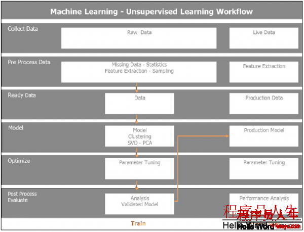
非監督式學習工作流程
?
與監督式學習相對,非監督式學習的初始數據使沒有標注的,這是真實生活的情形。通過聚類或降維算法提取數據中的結構, 在非監督式學習中,不用分割數據到訓練和測試中,由于數據沒有標注,我們不能做任何預測。訓練數據的6個步驟與監督式學習中的那些步驟類似。1旦模型訓練過了,將評估結果和調優模型,然后發布到生產環境。
非監督式學習是監督式學習的初始步驟。 也即是說, 數據降維先于進入學習階段。
非監督式機器學習的工作流程和數據流表達以下:
感受1下從Twitter提取到的數據,理解數據結構,然后運行 K-Means 聚類算法 . 使用非監督式的處理和數據流程,步驟以下:?
1. 組合所有的 tweet文件成1個 dataframe.
2. ?解析 tweets, 移除停詞,提取表情符號,提取URL, 并終究規范化詞 (如,轉化為小寫,移除標點符號和數字).
3. 特點提取包括以下步驟:
?∞ Tokenization: 將tweet的文本解析成單個的單詞或tokens
??∞ TF-IDF: 利用 TF-IDF 算法從文本分詞中創建特點向量
???∞ Hash TF-IDF: 利用哈希函數的TF-IDF?
4.運行 K-Means 聚類算法.?
5.評估 K-Means聚類的結果:?
∞ 界定 tweet 的成員關系 和聚類結果
?∞ 通過量維縮放和PCA算法履行降維分析到兩維?
?∞ 繪制聚類?
6.流水線:?
∞ 調優相干聚類K值數目?
∞ 丈量模型本錢?
∞ 選擇優化的模型
Python 有自己的 Scikit-Learn 機器學習庫,是最可靠直觀和硬朗的工具之1 。 使用Pandas 和 Scikit-Learn運行預處理和非監督式學習。 在用Spark MLlib 完成聚類之前,使用Scikit-Learn來探索數據的抽樣是非常有益的。這里混合了?7,540 tweets, 它包括了與Apache Spark,Python相干的tweets, 行將到來的總統選舉: 希拉里克林頓 和 唐納德 ,1些時尚相干的 tweets , Lady Gaga 和Justin Bieber的音樂. 在Twitter 數據集上使用?Scikit-Learn 并運行K-Means 聚類算法。
先將樣本數據加載到 1個 Pandas dataframe:?
import pandas as pd?
csv_in = 'C:\\Users\\Amit\\Documents\\IPython Notebooks\\AN00_Data\\?unq_tweetstxt.csv'?
twts_df01 = pd.read_csv(csv_in, sep =';', encoding='utf-8')? In [24]:
csv(csv_in, sep =';', encoding='utf-8') In [24]:?
twts_df01.count() Out[24]:
Unnamed: 0 7540 id 7540 created_at 7540 user_id 7540 user_name 7538 tweet_text 7540 dtype: int64
#
# Introspecting the tweets text
# In [82]:
twtstxt_ls01[6910:6920] Out[82]:
['RT @deroach_Ismoke: I am NOT voting for #hilaryclinton http://t.co/jaZZpcHkkJ', 'RT @AnimalRightsJen: #HilaryClinton What do Bernie Sanders and Donald Trump Have in Common?: He has so far been th... http://t.co/t2YRcGCh6…', 'I understand why Bill was out banging other chicks....... I mean
look at what he is married to.....\n@HilaryClinton',
'#HilaryClinton What do Bernie Sanders and Donald Trump Have in Common?: He has so far been th... http://t.co/t2YRcGCh67 #Tcot #UniteBlue']
先從Tweets 的文本中做1個特點提取,使用1個有10000特點和英文停詞的TF-IDF 矢量器將數據集向量化:
In [37]:
print("Extracting features from the training dataset using a sparse vectorizer")
t0 = time()
Extracting features from the training dataset using a sparse
vectorizer
In [38]:
vectorizer = TfidfVectorizer(max_df=0.5, max_features=10000,
min_df=2, stop_words='english',use_idf=True)
X = vectorizer.fit_transform(twtstxt_ls01) # Output of the TFIDF Feature vectorizer print("done in %fs" % (time() - t0))
print("n_samples: %d, n_features: %d" % X.shape)
print()
done in 5.232165s
n_samples: 7540, n_features: 6638
數據集被分成具有6638特點的7540個抽樣, 構成稀疏矩陣給 K-Means 聚類算法 ,初始選擇7個聚類和最多100次迭代:
In [47]:
km = KMeans(n_clusters=7, init='k-means++', max_iter=100, n_init=1,
verbose=1)
print("Clustering sparse data with %s" % km)
t0 = time()
km.fit(X)
print("done in %0.3fs" % (time() - t0))
Clustering sparse data with KMeans(copy_x=True, init='k-means++', max_iter=100, n_clusters=7, n_init=1,
n_jobs=1, precompute_distances='auto', random_state=None,
tol=0.0001,verbose=1)
Initialization complete
Iteration 0, inertia 13635.141 Iteration 1, inertia 6943.485 Iteration 2, inertia 6924.093 Iteration 3, inertia 6915.004 Iteration 4, inertia 6909.212 Iteration 5, inertia 6903.848 Iteration 6, inertia 6888.606 Iteration 7, inertia 6863.226 Iteration 8, inertia 6860.026 Iteration 9, inertia 6859.338 Iteration 10, inertia 6859.213 Iteration 11, inertia 6859.102 Iteration 12, inertia 6859.080 Iteration 13, inertia 6859.060 Iteration 14, inertia 6859.047 Iteration 15, inertia 6859.039 Iteration 16, inertia 6859.032 Iteration 17, inertia 6859.031 Iteration 18, inertia 6859.029 Converged at iteration 18 done in 1.701s
在18次迭代后 K-Means聚類算法收斂,根據相應的關鍵詞看1下7個聚類的結果 . Clusters 0 和6 是關于音樂和時尚的 Justin Bieber 和Lady Gaga 相干的tweets.
Clusters 1 和5 是與美國總統大選 Donald Trump和 Hilary Clinton相干的tweets. Clusters 2 和3 是我們感興趣的Apache Spark 和Python. Cluster 4 包括了 Thailand相干的 tweets:
In [49]:
print("Top terms per cluster:")
order_centroids = km.cluster_centers_.argsort()[:, ::-1]
terms = vectorizer.get_feature_names() for i in range(7):
print("Cluster %d:" % i, end='') for ind in order_centroids[i, :20]:
print(' %s' % terms[ind], end='') print()
Top terms per cluster:
Cluster 0: justinbieber love mean rt follow thank hi https whatdoyoumean video wanna hear whatdoyoumeanviral rorykramer happy lol making person dream justin
Cluster 1: donaldtrump hilaryclinton rt https trump2016
realdonaldtrump trump gop amp justinbieber president clinton emails oy8ltkstze tcot like berniesanders hilary people email
Cluster 2: bigdata apachespark hadoop analytics rt spark training chennai ibm datascience apache processing cloudera mapreduce data sap https vora transforming development
Cluster 3: apachespark python https rt spark data amp databricks using new learn hadoop ibm big apache continuumio bluemix learning join open Cluster 4: ernestsgantt simbata3 jdhm2015 elsahel12 phuketdailynews dreamintentions beyhiveinfrance almtorta18 civipartnership 9_a_6 25whu72ep0 k7erhvu7wn fdmxxxcm3h osxuh2fxnt 5o5rmb0xhp jnbgkqn0dj ovap57ujdh dtzsz3lb6x sunnysai12345 sdcvulih6g
Cluster 5: trump donald donaldtrump starbucks trumpquote
trumpforpresident oy8ltkstze https zfns7pxysx silly goy stump trump2016 news jeremy coffee corbyn ok7vc8aetz rt tonight
Cluster 6: ladygaga gaga lady rt https love follow horror cd story ahshotel american japan hotel human trafficking music fashion diet queen ahs
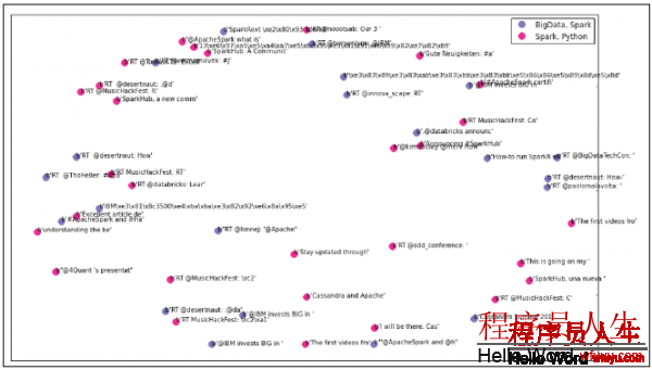
我們將通過畫圖來可視化結果。由于我們有6638個特點的7540個抽樣,很難多維可視化,所以通過MDS算法來降維描繪 :
import matplotlib.pyplot as plt
import matplotlib as mpl
from sklearn.manifold import MDS
MDS() # # Bring down the MDS to two dimensions (components) as we will plot the clusters # mds = MDS(n_components=2, dissimilarity="precomputed", random_state=1)
pos = mds.fit_transform(dist) # shape (n_components, n_samples)
xs, ys = pos[:, 0], pos[:, 1]
In [67]: # # Set up colors per clusters using a dict # cluster_colors = {0: '#1b9e77', 1: '#d95f02', 2: '#7570b3', 3:'#e7298a', 4: '#66a61e', 5: '#9990b3', 6: '#e8888a'} # #set up cluster names using a dict # cluster_names = {0: 'Music, Pop', 1: 'USA Politics, Election', 2: 'BigData, Spark', 3: 'Spark, Python', 4: 'Thailand', 5: 'USA Politics, Election', 6: 'Music, Pop'}
In [115]: # # ipython magic to show the matplotlib plots inline # %matplotlib inline # # Create data frame which includes MDS results, cluster numbers and tweet texts to be displayed # df = pd.DataFrame(dict(x=xs, y=ys, label=clusters, txt=twtstxt_ls02_
utf8))
ix_start = 2000 ix_stop = 2050 df01 = df[ix_start:ix_stop]
print(df01[['label','txt']])
print(len(df01))
print() # Group by cluster groups = df.groupby('label')
groups01 = df01.groupby('label') # Set up the plot fig, ax = plt.subplots(figsize=(17, 10))
ax.margins(0.05) # # Build the plot object # for name, group in groups01:
ax.plot(group.x, group.y, marker='o', linestyle='', ms=12,
label=cluster_names[name], color=cluster_colors[name],
mec='none')
ax.set_aspect('auto')
ax.tick_params(\
axis= 'x', # settings for x-axis
which='both', #
bottom='off', #
top='off', #
labelbottom='off')
ax.tick_params(\
axis= 'y', # settings for y-axis
which='both', #
left='off', #
top='off', #
labelleft='off')
ax.legend(numpoints=1) # # # Add label in x,y position with tweet text # for i in range(ix_start, ix_stop):
ax.text(df01.ix[i]['x'], df01.ix[i]['y'], df01.ix[i]['txt'],
size=10)
plt.show() # Display the plot
label text 2000 2 b'RT @BigDataTechCon: ' 2001 3 b"@4Quant 's presentat" 2002 2 b'Cassandra Summit 201'
這是Cluster 2的圖, 由藍點表示Big Data 和 Spark; Cluster 3, 由紅點表示Spark 和Python,和相干的 tweets 內容抽樣 :
利用 Scikit-Learn 的處理結果,已探索到數據的1些好的見解,現在關注在Twitter數據集上履行 Spark MLlib。
預處理數據集
為了準備在數據集上運行聚類算法,現在聚焦特點提取和工程化。我們實例化Spark Context,讀取 Twitter 數據集到1個 Spark dataframe. 然后,對tweet文本數據連續分詞,利用哈希詞頻算法到 tokens, 并終究利用 Inverse Document Frequency 算法,重新縮放數據 。代碼以下:
In [3]: import pandas as pd
csv_in = '/home/an/spark/spark⑴.5.0-bin-hadoop2.6/examples/AN_Spark/data/unq_tweetstxt.csv' pddf_in = pd.read_csv(csv_in, index_col=None, header=0, sep=';',encoding='utf⑻')
In [4]:
sqlContext = SQLContext(sc)
In [5]: spdf_02 = sqlContext.createDataFrame(pddf_in[['id', 'user_id', 'user_name', 'tweet_text']])
In [8]:
spdf_02.show()
In [7]:
spdf_02.take(3)
Out[7]:
[Row(id=638830426971181057, user_id=3276255125, user_name=u'True Equality', tweet_text=u'ernestsgantt: BeyHiveInFrance: 9_A_6:dreamintentions: elsahel12: simbata3: JDHM2015: almtorta18:dreamintentions:\u2026 http://t.co/VpD7FoqMr0'),
Row(id=638830426727911424, user_id=3276255125, user_name=u'True
Equality', tweet_text=u'ernestsgantt: BeyHiveInFrance:
PhuketDailyNews: dreamintentions: elsahel12: simbata3: JDHM2015:almtorta18: CiviPa\u2026 http://t.co/VpD7FoqMr0'),
Row(id=638830425402556417, user_id=3276255125, user_name=u'True
Equality', tweet_text=u'ernestsgantt: BeyHiveInFrance: 9_A_6:
ernestsgantt: elsahel12: simbata3: JDHM2015: almtorta18:
CiviPartnership: dr\u2026 http://t.co/EMDOn8chPK')]
In [9]: from pyspark.ml.feature import HashingTF, IDF, Tokenizer
In [10]: tokenizer = Tokenizer(inputCol="tweet_text",outputCol="tokens")
tokensData = tokenizer.transform(spdf_02)
In [11]:
tokensData.take(1)
Out[11]:
[Row(id=638830426971181057, user_id=3276255125, user_name=u'True Equality', tweet_text=u'ernestsgantt: BeyHiveInFrance:9_A_6: dreamintentions: elsahel12: simbata3: JDHM2015:almtorta18: dreamintentions:\u2026 http://t.co/VpD7FoqMr0',
tokens=[u'ernestsgantt:', u'beyhiveinfrance:', u'9_a_6:', u'dreamintentions:', u'elsahel12:', u'simbata3:', u'jdhm2015:',u'almtorta18:', u'dreamintentions:\u2026', u'http://t.co/vpd7foqmr0'])]
In [14]: hashingTF = HashingTF(inputCol="tokens", outputCol="rawFeatures",numFeatures=2000)
featuresData = hashingTF.transform(tokensData)
In [15]:
featuresData.take(1)
Out[15]:
[Row(id=638830426971181057, user_id=3276255125, user_name=u'True Equality', tweet_text=u'ernestsgantt: BeyHiveInFrance:9_A_6: dreamintentions: elsahel12: simbata3: JDHM2015:almtorta18: dreamintentions:\u2026 http://t.co/VpD7FoqMr0',
tokens=[u'ernestsgantt:', u'beyhiveinfrance:', u'9_a_6:', u'dreamintentions:', u'elsahel12:', u'simbata3:', u'jdhm2015:',u'almtorta18:', u'dreamintentions:\u2026', u'http://t.co/vpd7foqmr0'],
rawFeatures=SparseVector(2000, {74: 1.0, 97: 1.0, 100: 1.0, 160: 1.0,185: 1.0, 742: 1.0, 856: 1.0, 991: 1.0, 1383: 1.0, 1620: 1.0}))]
In [16]: idf = IDF(inputCol="rawFeatures", outputCol="features")
idfModel = idf.fit(featuresData)
rescaledData = idfModel.transform(featuresData) for features in rescaledData.select("features").take(3):
print(features)
In [17]:
rescaledData.take(2)
Out[17]:
[Row(id=638830426971181057, user_id=3276255125, user_name=u'True Equality', tweet_text=u'ernestsgantt: BeyHiveInFrance:9_A_6: dreamintentions: elsahel12: simbata3: JDHM2015:almtorta18: dreamintentions:\u2026 http://t.co/VpD7FoqMr0',
tokens=[u'ernestsgantt:', u'beyhiveinfrance:', u'9_a_6:', u'dreamintentions:', u'elsahel12:', u'simbata3:', u'jdhm2015:',u'almtorta18:', u'dreamintentions:\u2026', u'http://t.co/vpd7foqmr0'],
rawFeatures=SparseVector(2000, {74: 1.0, 97: 1.0, 100: 1.0, 160:1.0, 185: 1.0, 742: 1.0, 856: 1.0, 991: 1.0, 1383: 1.0, 1620: 1.0}),
features=SparseVector(2000, {74: 2.6762, 97: 1.8625, 100: 2.6384, 160:2.9985, 185: 2.7481, 742: 5.5269, 856: 4.1406, 991: 2.9518, 1383:4.694, 1620: 3.073})),
Row(id=638830426727911424, user_id=3276255125, user_name=u'True
Equality', tweet_text=u'ernestsgantt: BeyHiveInFrance:
PhuketDailyNews: dreamintentions: elsahel12: simbata3:
JDHM2015: almtorta18: CiviPa\u2026 http://t.co/VpD7FoqMr0',
tokens=[u'ernestsgantt:', u'beyhiveinfrance:', u'phuketdailynews:',u'dreamintentions:', u'elsahel12:', u'simbata3:', u'jdhm2015:',u'almtorta18:', u'civipa\u2026', u'http://t.co/vpd7foqmr0'],
rawFeatures=SparseVector(2000, {74: 1.0, 97: 1.0, 100: 1.0, 160:1.0, 185: 1.0, 460: 1.0, 987: 1.0, 991: 1.0, 1383: 1.0, 1620: 1.0}),
features=SparseVector(2000, {74: 2.6762, 97: 1.8625, 100: 2.6384,160: 2.9985, 185: 2.7481, 460: 6.4432, 987: 2.9959, 991: 2.9518, 1383:4.694, 1620: 3.073}))]
In [21]:
rs_pddf = rescaledData.toPandas()
In [22]:
rs_pddf.count()
Out[22]:
id 7540 user_id 7540 user_name 7540 tweet_text 7540 tokens 7540 rawFeatures 7540 features 7540 dtype: int64
In [27]:
feat_lst = rs_pddf.features.tolist()
In [28]:
feat_lst[:2]
Out[28]:
[SparseVector(2000, {74: 2.6762, 97: 1.8625, 100: 2.6384, 160: 2.9985,185: 2.7481, 742: 5.5269, 856: 4.1406, 991: 2.9518, 1383: 4.694, 1620: 3.073}),
SparseVector(2000, {74: 2.6762, 97: 1.8625, 100: 2.6384, 160: 2.9985,185: 2.7481, 460: 6.4432, 987: 2.9959, 991: 2.9518, 1383: 4.694, 1620:3.073})]
運行聚類算法
在Twitter數據集上運行 K-Means 算法, 作為非標簽的tweets, 希望看到Apache Spark tweets 構成1個聚類。 遵從之前的步驟, 特點的 TF-IDF 稀疏向量轉化為1個 RDD 將被輸入到 Spark MLlib 程序。初始化 K-Means 模型為 5 聚類, 10 次迭代:
In [32]: from pyspark.mllib.clustering import KMeans, KMeansModel from numpy import array from math import sqrt
In [34]: in_Data = sc.parallelize(feat_lst)
In [35]:
in_Data.take(3)
Out[35]:
[SparseVector(2000, {74: 2.6762, 97: 1.8625, 100: 2.6384, 160: 2.9985,185: 2.7481, 742: 5.5269, 856: 4.1406, 991: 2.9518, 1383: 4.694, 1620:3.073}),
SparseVector(2000, {74: 2.6762, 97: 1.8625, 100: 2.6384, 160: 2.9985,185: 2.7481, 460: 6.4432, 987: 2.9959, 991: 2.9518, 1383: 4.694, 1620:3.073}),
SparseVector(2000, {20: 4.3534, 74: 2.6762, 97: 1.8625, 100: 5.2768,185: 2.7481, 856: 4.1406, 991: 2.9518, 1039: 3.073, 1620: 3.073, 1864:4.6377})]
In [37]:
in_Data.count()
Out[37]: 7540 In [38]: clusters = KMeans.train(in_Data, 5, maxIterations=10,
runs=10, initializationMode="random")
In [53]: def error(point): center = clusters.centers[clusters.predict(point)] return sqrt(sum([x**2 for x in (point - center)]))
WSSSE = in_Data.map(lambda point: error(point)).reduce(lambda x, y: x + y)
print("Within Set Sum of Squared Error = " + str(WSSSE))
評估模型和結果
聚類算法調優的1個方式是改變聚類的個數并驗證輸出. 檢查這些聚類,感受1下目前的聚類結果:
In [43]:
cluster_membership = in_Data.map(lambda x:clusters.predict(x)) In [54]:
cluster_idx = cluster_membership.zipWithIndex() In [55]: type(cluster_idx) Out[55]:
pyspark.rdd.PipelinedRDD In [58]:
cluster_idx.take(20) Out[58]:
[(3, 0),
(3, 1),
(3, 2),
(3, 3),
(3, 4),
(3, 5),
(1, 6),
(3, 7),
(3, 8),
(3, 9),
(3, 10),
(3, 11),
(3, 12),
(3, 13),
(3, 14),
(1, 15),
(3, 16),
(3, 17),
(1, 18),
(1, 19)] In [59]:
cluster_df = cluster_idx.toDF() In [65]:
pddf_with_cluster = pd.concat([pddf_in, cluster_pddf],axis=1) In [76]:
pddf_with_cluster._1.unique() Out[76]: array([3, 1, 4, 0, 2]) In [79]:
pddf_with_cluster[pddf_with_cluster['_1'] == 0].head(10) Out[79]:
Unnamed: 0 id created_at user_id user_name tweet_text _1 _2 6227 3 642418116819988480 Fri Sep 11 19:23:09 +0000 2015 49693598 Ajinkya Kale RT @bigdata: Distributed Matrix Computations
i... 0 6227 6257 45 642391207205859328 Fri Sep 11 17:36:13 +0000 2015 937467860 Angela Bassa [Auto] I'm reading ""Distributed Matrix
Comput... 0 6257
6297 119 642348577147064320 Fri Sep 11 14:46:49 +0000
2015 18318677 Ben Lorica Distributed Matrix Computations in @
ApacheSpar... 0 6297
In [80]:
pddf_with_cluster[pddf_with_cluster['_1'] == 1].head(10)
Out[80]:
Unnamed: 0 id created_at user_id user_name tweet_text _1
_2
6 6 638830419090079746 Tue Sep 01 21:46:55 +0000 2015
2241040634 Massimo Carrisi Python:Python: Removing \xa0 from
string? - I ... 16
15 17 638830380578045953 Tue Sep 01 21:46:46 +0000 2015
57699376 Rafael Monnerat RT @ramalhoorg: Noite de autógrafos do
Fluent ... 115
18 41 638830280988426250 Tue Sep 01 21:46:22 +0000 2015
951081582 Jack Baldwin RT @cloudaus: We are 3/4 full! 2-day @
swcarpen... 1 18
19 42 638830276626399232 Tue Sep 01 21:46:21 +0000 2015
6525302 Masayoshi Nakamura PynamoDB #AWS #DynamoDB #Python
http://... 1 19
20 43 638830213288235008 Tue Sep 01 21:46:06 +0000 2015
3153874869 Baltimore Python Flexx: Python UI tookit based on web
technolog... 1 20
21 44 638830117645516800 Tue Sep 01 21:45:43 +0000 2015
48474625 Radio Free Denali Hmm, emerge --depclean wants to remove
somethi... 1 21
22 46 638829977014636544 Tue Sep 01 21:45:10 +0000 2015
154915461 Luciano Ramalho Noite de autógrafos do Fluent Python no
Garoa ... 122
23 47 638829882928070656 Tue Sep 01 21:44:47 +000