
Stanford機器學習課程的主頁是: http://cs229.stanford.edu/
主講人Andrew Ng是機器學習界的大牛,創辦最大的公然課網站coursera,前段時間還聽說加入了百度。他講的機器學習課程可謂每一個學計算機的人必看。全部課程的大綱大致以下:
本筆記主要是關于Linear Regression和Logistic Regression部份的學習實踐記錄。
舉了1個房價預測的例子,
| Area(feet^2) | #bedrooms | Price(1000$) |
|---|---|---|
| 2014 | 3 | 400 |
| 1600 | 3 | 330 |
| 2400 | 3 | 369 |
| 1416 | 2 | 232 |
| 3000 | 4 | 540 |
| 3670 | 4 | 620 |
| 4500 | 5 | 800 |
Assume:房價與“面積和臥室數量”是線性關系,用線性關系進行放假預測。因此給出線性模型, hθ(x)?=?∑θTx ,其中 x?=?[x1,?x2] , 分別對應面積和臥室數量。 為得到預測模型,就應當根據表中已有的數據擬合得到參數 θ 的值。課程通過從幾率角度進行解釋(主要用到了大數定律即“線性擬合模型的誤差滿足高斯散布”的假定,通過最大似然求導就可以得到下面的表達式)為何應當求解以下的最小2乘表達式來到達求解參數的目的,
上述 J(θ) 稱為cost function, 通過 minJ(θ) 便可得到擬合模型的參數。
解 minJ(θ) 的方法有多種, 包括Gradient descent algorithm和Newton's method,這兩種都是運籌學的數值計算方法,非常合適計算機運算,這兩種算法不但合適這里的線性回歸模型,對非線性模型以下面的Logistic模型也適用。除此以外,Andrew Ng還通過線性代數推導了最小均方的算法的閉合數學情勢,
Gradient descent algorithm履行進程中又分兩種方法:batch gradient descent和stochastic gradient descent。batch gradient descent每次更新 θ 都用到所有的樣本數據,而stochastic gradient descent每次更新則都僅用單個的樣本數據。二者更新進程以下:
batch gradient descent
stochastic gradient descent
for i=1 to m
二者只不過1個將樣本放在了for循環上,1者放在了。事實證明,只要選擇適合的學習率 α , Gradient descent algorithm總是能收斂到1個接近最優值的值。學習率選擇過大可能造成cost function的發散,選擇太小,收斂速度會變慢。
關于收斂條件,Andrew Ng沒有在課程中提到更多,我給出兩種收斂準則:
下面是使用batch gradient descent擬合上面房價問題的例子,
clear all;
clc

%% 原數據
x = [2014, 1600, 2400, 1416, 3000, 3670, 4500;...
    3,3,3,2,4,4,5;];
y = [400 330 369 232 540 620 800];

error = Inf;
threshold = 4300;
alpha = 10^(-10);
x = [zeros(1,size(x,2)); x];  % x0 = 0,擬合常數項
theta = [0;0;0]; % 常數項為0
J = 1/2*sum((y-theta'*x).^2);
costs = [];
while error > threshold
    tmp = y-theta'*x;
    theta(1) = theta(1) + alpha*sum(tmp.*x(1,:));
    theta(2) = theta(2) + alpha*sum(tmp.*x(2,:));
    theta(3) = theta(3) + alpha*sum(tmp.*x(3,:));
%     J_last = J;
    J = 1/2*sum((y-theta'*x).^2);
%     error = abs(J-J_last);
    error = J;
    costs =[costs, error];
end

%% 繪制
figure,
subplot(211);
plot3(x(2,:),x(3,:),y, '*');
grid on;
xlabel('Area');
ylabel('#bedrooms');
zlabel('Price(1000$)');

hold on;
H = theta'*x;
plot3(x(2,:),x(3,:),H,'r*');

hold on
hx(1,:) = zeros(1,20);
hx(2,:) = 1000:200:4800;
hx(3,:) = 1:20;
[X,Y] = meshgrid(hx(2,:), hx(3,:));
H = theta(2:3)'*[X(:)'; Y(:)'];
H = reshape(H,[20,20]);
mesh(X,Y,H);

legend('原數據', '對原數據的擬合', '擬合平面');

subplot(212);
plot(costs, '.-');
grid on
title('error=J(	heta)的迭代收斂進程');
xlabel('迭代次數');
ylabel('J(	heta)');
擬合及收斂進程以下:
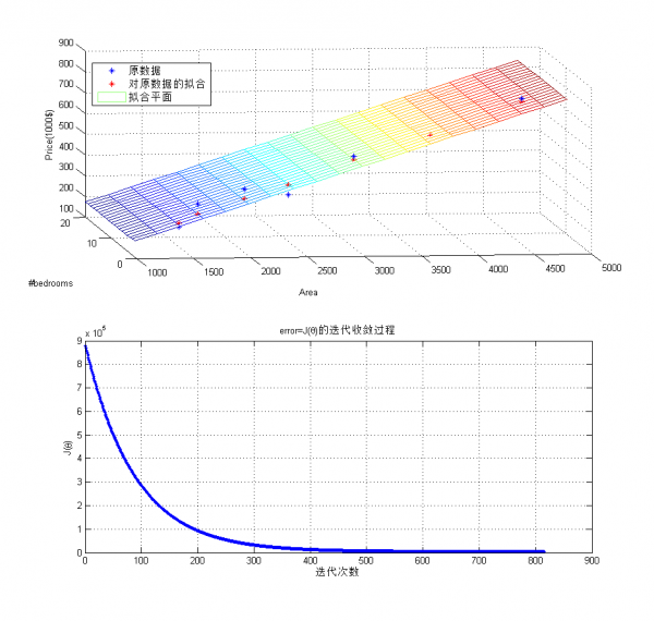
不論是梯度降落,還是線性回歸模型,都是工具!!分析結果更重要,從上面的擬合平面可以看到,影響房價的主要因素是面積而非臥室數量。
很多情況下,模型其實不是線性的,比如股票隨時間的漲跌進程。這類情況下, hθ(x)?=?θTx 的假定不再成立。此時,有兩種方案:
其中權值的1種好的選擇方式是:
Linear Regression解決的是連續的預測和擬合問題,而Logistic Regression解決的是離散的分類問題。兩種方式,但本質殊途同歸,二者都可以算是指數函數族的特例。
在分類問題中,y取值在{0,1}之間,因此,上述的Liear Regression明顯不適應。修改模型以下
該模型稱為Logistic函數或Sigmoid函數。為何選擇該函數,我們看看這個函數的圖形就知道了,
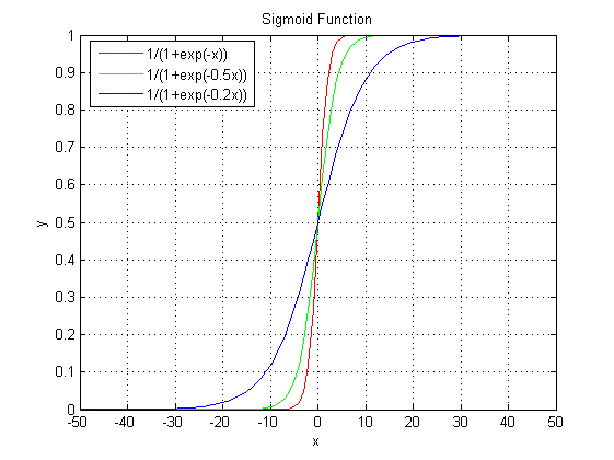
Sigmoid函數范圍在[0,1]之間,參數 θ 只不過控制曲線的峻峭程度。以0.5為截點,>0.5則y值為1,< 0.5則y值為0,這樣就實現了兩類分類的效果。
假定 P(y?=?1|x;?θ)?=?hθ(x) , P(y?=?0|x;?θ)?=?1???hθ(x) , 寫得更緊湊1些,
對m個訓練樣本,使其似然函數最大,則有
一樣的可以用梯度降落法求解上述的最大值問題,只要將最大值求解轉化為求最小值,則迭代公式1模1樣,
最后的梯度降落方式和Linear Regression1致。我做了個例子(數據集鏈接),下面是Logistic的Matlab代碼,
function Logistic

clear all;
close all
clc

data = load('LogisticInput.txt');
x = data(:,1:2);
y = data(:,3);

% Plot Original Data
figure,
positive = find(y==1);
negtive = find(y==0);
hold on
plot(x(positive,1), x(positive,2), 'k+', 'LineWidth',2, 'MarkerSize', 7);
plot(x(negtive,1), x(negtive,2), 'bo', 'LineWidth',2, 'MarkerSize', 7);

% Compute Likelihood(Cost) Function
[m,n] = size(x);
x = [ones(m,1) x];
theta = zeros(n+1, 1);
[cost, grad] = cost_func(theta, x, y);
threshold = 0.1;
alpha = 10^(⑴);
costs = [];
while cost > threshold
    theta = theta + alpha * grad;
    [cost, grad] = cost_func(theta, x, y);
    costs = [costs cost];
end

% Plot Decision Boundary
hold on
plot_x = [min(x(:,2))⑵,max(x(:,2))+2];
plot_y = (⑴./theta(3)).*(theta(2).*plot_x + theta(1));
plot(plot_x, plot_y, 'r-');
legend('Positive', 'Negtive', 'Decision Boundary')
xlabel('Feature Dim1');
ylabel('Feature Dim2');
title('Classifaction Using Logistic Regression');

% Plot Costs Iteration
figure,
plot(costs, '*');
title('Cost Function Iteration');
xlabel('Iterations');
ylabel('Cost Fucntion Value');

end

function g=sigmoid(z)
g = 1.0 ./ (1.0+exp(-z));
end

function [J,grad] = cost_func(theta, X, y)
% Computer Likelihood Function and Gradient
m = length(y); % training examples
hx = sigmoid(X*theta);
J = (1./m)*sum(-y.*log(hx)-(1.0-y).*log(1.0-hx));
grad = (1./m) .* X' * (y-hx);
end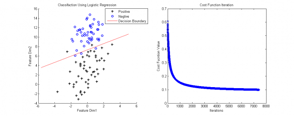
判決邊界(Decesion Boundary)的計算是令h(x)=0.5得到的。當輸入新的數據,計算h(x):h(x)>0.5為正樣本所屬的類,h(x)< 0.5 為負樣本所屬的類。
這部份在Andrew Ng課堂上沒有講,參考了網絡上的資料。
上面的數據可以通過直線進行劃分,但實際中存在那末種情況,沒法直接使用直線判決邊界(看后面的例子)。
為解決上述問題,必須將特點映照到高維,然后通過非直線判決界面進行劃分。特點映照的方法將已有的特點進行多項式組合,構成更多特點,
上面將2維特點映照到了2階(還可以映照到更高階),這便于構成非線性的判決邊界。
但還存在問題,雖然上面方法便于對非線性的數據進行劃分,但也容易由于高維特性造成過擬合。因此,引入泛化項應對過擬合問題。似然函數添加泛化項后變成,
此時梯度降落算法產生改變,
最后來個例子,樣本數據鏈接,對應的含泛化項和特點映照的matlab分類代碼以下:
function LogisticEx2

clear all;
close all
clc

data = load('ex2data2.txt');
x = data(:,1:2);
y = data(:,3);

% Plot Original Data
figure,
positive = find(y==1);
negtive = find(y==0);
subplot(1,2,1);
hold on
plot(x(positive,1), x(positive,2), 'k+', 'LineWidth',2, 'MarkerSize', 7);
plot(x(negtive,1), x(negtive,2), 'bo', 'LineWidth',2, 'MarkerSize', 7);

% Compute Likelihood(Cost) Function
[m,n] = size(x);
x = mapFeature(x);
theta = zeros(size(x,2), 1);
lambda = 1;
[cost, grad] = cost_func(theta, x, y, lambda);
threshold = 0.53;
alpha = 10^(-1);
costs = [];
while cost > threshold
    theta = theta + alpha * grad;
    [cost, grad] = cost_func(theta, x, y, lambda);
    costs = [costs cost];
end

% Plot Decision Boundary
hold on
plotDecisionBoundary(theta, x, y);
legend('Positive', 'Negtive', 'Decision Boundary')
xlabel('Feature Dim1');
ylabel('Feature Dim2');
title('Classifaction Using Logistic Regression');

% Plot Costs Iteration
% figure,
subplot(1,2,2);plot(costs, '*');
title('Cost Function Iteration');
xlabel('Iterations');
ylabel('Cost Fucntion Value');

end

function f=mapFeature(x)
% Map features to high dimension
degree = 6;
f = ones(size(x(:,1)));
for i = 1:degree
    for j = 0:i
        f(:, end+1) = (x(:,1).^(i-j)).*(x(:,2).^j);
    end
end
end

function g=sigmoid(z)
g = 1.0 ./ (1.0+exp(-z));
end

function [J,grad] = cost_func(theta, X, y, lambda)
% Computer Likelihood Function and Gradient
m = length(y); % training examples
hx = sigmoid(X*theta);
J = (1./m)*sum(-y.*log(hx)-(1.0-y).*log(1.0-hx)) + (lambda./(2*m)*norm(theta(2:end))^2);
regularize = (lambda/m).*theta;
regularize(1) = 0;
grad = (1./m) .* X' * (y-hx) - regularize;
end

function plotDecisionBoundary(theta, X, y)
%PLOTDECISIONBOUNDARY Plots the data points X and y into a new figure with
%the decision boundary defined by theta
%   PLOTDECISIONBOUNDARY(theta, X,y) plots the data points with + for the
%   positive examples and o for the negative examples. X is assumed to be
%   a either
%   1) Mx3 matrix, where the first column is an all-ones column for the
%      intercept.
%   2) MxN, N>3 matrix, where the first column is all-ones

% Plot Data
% plotData(X(:,2:3), y);
hold on

if size(X, 2) <= 3
    % Only need 2 points to define a line, so choose two endpoints
    plot_x = [min(X(:,2))-2,  max(X(:,2))+2];

    % Calculate the decision boundary line
    plot_y = (-1./theta(3)).*(theta(2).*plot_x + theta(1));

    % Plot, and adjust axes for better viewing
    plot(plot_x, plot_y)

    % Legend, specific for the exercise
    legend('Admitted', 'Not admitted', 'Decision Boundary')
    axis([30, 100, 30, 100])
else
    % Here is the grid range
    u = linspace(-1, 1.5, 50);
    v = linspace(-1, 1.5, 50);

    z = zeros(length(u), length(v));
    % Evaluate z = theta*x over the grid
    for i = 1:length(u)
        for j = 1:length(v)
            z(i,j) = mapFeature([u(i), v(j)])*theta;
        end
    end
    z = z'; % important to transpose z before calling contour

    % Plot z = 0
    % Notice you need to specify the range [0, 0]
    contour(u, v, z, [0, 0], 'LineWidth', 2)
end
end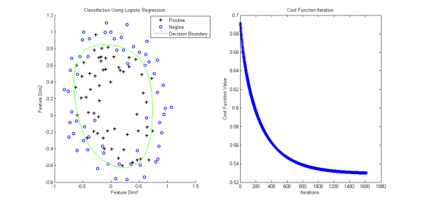
我們再回過頭來看Logistic問題:對非線性的問題,只不過使用了1個叫Sigmoid的非線性映照成1個線性問題。那末,除Sigmoid函數,還有其它的函數可用嗎?Andrew Ng老師還講了指數函數族。

上一篇 IP 分片丟失重傳
程序員人生,我編程,我富裕,記住wfuyu網,php教程,php學習,php手冊,CMS模版制作
聲明:本站大部分內容是作者原創,少部分收集于互聯網供大家一起學習,原版權很多不明,如有侵權請聯系本站,謝謝!
粵ICP備14040726號-1?? 2015-2020 程序員人生 版權所有


